A Study on Intuitive Technique of Risk Assessment for Route of Ships Transporting Hazardous and Noxious Substances

2.1 The scope of maritime traffic accidents and risk of routes by ships carrying HNS

The definition of risk can vary depending on the elements to be evaluated, application areas, and intended purposes. Generally, risk could be the product of probability and consequences in a mathematical model (Cho et al., 2013; EmSA, 2007; ImO, 2002). In this study, to focus on the prevention of accidents of ships carrying HNS while navigation at sea, we assumed that consequential components of navigational accident risks were considered at the same level as a constant factor; thus, the maritime traffic risks have been defined as a probability of designated types of maritime traffic accidents in a certain area.

For the maritime traffic accidents, the scope of this study was circumscribed to accidents related to navigation of ships transporting HNS such as grounding, contact, capsizing, and sinking resulting from hazards existing in the external environments and exceeding the permissible range of the maritime traffic risk, to assess the route risk at the stage of planning the course without consideration of dynamic objects such as other ships with fluctuant data throughout real-time. Therefore, this study mainly assessed factors reflecting the surrounding environment of the region where the ship is heading.

2.2 The concept of risk contour

Normally, a contour map, which is known as a topographic line map, is a representation of the horizontal cross section of the Earth’s surface (Cronin, 1995; Li and Sui, 2000). Although most topographical maps or nautical charts are represented in contour in order to describe and visualize the altitude of lands or the depth of waters, the risk contour is suggested in this study so that the navigating officer or the person managing the vessel can easily understand the degree of risks along the ship’s route and make a reasonable decision as the development of the previous study’s hazard contour (Jeong et al., 2017). The risk contour was introduced as the plotted map that connects the same risk areas, to be overlaid on the electronic charts as making the degree of risks visible.

2.3 The purpose and advantage of risk contour

There are significant advantages in using the risk contour when the route is evaluated. First of all, the risk contour reflects the scattered and separate data in the region and eventually generate the continuous information as continuous lines. Secondly, instead of using qualitative conventional navigation, the risk contour can quantitatively evaluate the risk of the route of ships carrying HNS; thus the operator can visualize and intuitively understand the situation. This allows the operator to make reasonable decisions based on the circumstances and avoid or minimize the risk of the route. In addition, risk contours offer new types of information such as the risk sum of the total route, changing trends, and distribution of the route risk. This is similar to the information offered by the topographical contour maps, which indicate that the area is steep when the contours are closely packed, and the area is flat when they are far apart (Cronin, 1995).

3.1 Determination of route risk factors

Several factors were defined in this study as variables causing maritime traffic accidents such as grounding, contact, capsizing and sinking. These factors were determined by reviewing previous studies, publications, past maritime traffic accident data, brain storming, and exchange of opinions with experts in the field (Swift, 1993; ImO, 2002; NImA, 2002; IALA, 2009; Kim and Lee, 2012; Lee and Kim 2013). Then, in accordance with the definition and the scope of maritime traffic risk in this study, the route risk factors were structured, as shown in Fig. 1.

Fig. 1.

Categories of maritime traffic risk factor and their attribute analysis

The external factors other than internal factors such as ship-born risks or human-generated risks were analyzed, and they can be divided into three major categories: absolute danger, absolute factor, and influential factor. Then, each of the major categories is specified in details. The water depth below the ship’s maximum draft including squat is defined as absolute danger. The least depth above the ship’s maximum draft including squat, natural obstacles like a wreck, rock, obstruction existing in the natural navigational environment, and artificial obstacles like a buoy, lighthouse, fishing ground, impediment made by human are all defined as absolute factors. meanwhile, the weather related conditions such as wind, current, and visibility are the influential factors. Finally, it was revealed that each factor in the detailed categories has its attribute of variability depending on time and/or position. For instance, the attributes of natural and artificial obstacles are dependent only on the position, because they are expressed differently in the location, and they do not change as time elapses in the fixed location.

3.2 Designation of route risk assessment area

Based on the factors affecting the route risk, the route risk assessment areas are designated as circular shapes reflecting the concept of position fixing interval that ships are practically using (OCImF, 2016). In other words, as the position fixing interval ensures that the ship will not encounter any hazards during the specific period of time, the risks can be assessed within circular areas plotted by specific intervals, as per the ship’s navigational safety. Additionally, the radius of circular units is the distance obtained by multiplying the position fixing interval and the ship’s transit speed. Fig. 3 represents a conceptual diagram of route risk assessment area within a region.

Fig. 3.

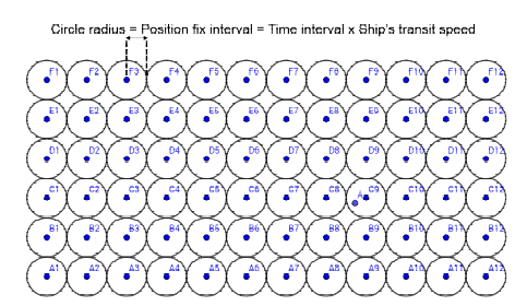
Conceptual diagram of the route assessment area and its relationship to position fixing interval

3.3 Algorithm for route risk assessment

The flow chart shown in Fig. 2 illustrates the algorithm developed to evaluate the route risk of ships carrying HNS. As a precondition, departure and the arrival point of the region should be identified to assess the route risk; thus, these points would be included in the region when the risk assessment is conducted.

Fig. 2.

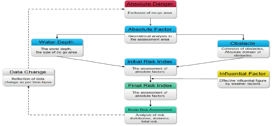
Flowchart of the quantitative route risk assessment using risk factors

First, the absolute danger, which is referred to as No Go Area in this study, is derived by comparing the water depth reflecting tidal height at the specific time and the ship’s maximum draft, including its squat. Then, the absolute danger areas are excluded; thus, the remaining area is considered safe for the ship to transit. Later, the absolute factors, i.e., the least depth more than the ship’s maximum draft and obstacles composed of natural or artificial elements, are evaluated, as shown in Table 1. In this stage, the least water depth is compared to the ship’s maximum draft, and the ratio between the depth and draft is entered to derive a relevant index. This index is multiplied by the incremental coefficient calculated from the size of No Go Area. Similarly, the obstacles are analyzed to determine the index based on the cohesion of their distribution within each area, and the index is multiplied by the incremental coefficient calculated from the absolute domain nearby obstacles. more details about measuring the obstacles considered as absolute factors are explained below. Then, risk assessment is performed in each circular area in terms of absolute factors, and the final risk can be computed considering the influential factors derived from analyzing the weather conditions. Finally, the induced values which were rounded off for the risk contour plot and intuitive analysis are obtained. As a result, a risk contour map can be visualized and route risk assessment can be conducted by analyzing the risk distribution of the route, distance, and total cumulative risk along the route based on the route plan. If data affecting the risk factors change, the algorithm will adjust the results to reflect the change. For example, the No Go Areas can vary according to the ship’s speed, draft, and tidal window, and the feedback allows to correctly adjust the results by reflecting the change. Fig. 3

Table 1

Matrix of rating criteria for risk factors

3.3.2 Obstacle assessment

Two categories of obstacles are defined in this study. One category includes the natural obstacles such as wrecks, rocks, and obstructions present in nature. While the other involves the artificial obstacle such as buoys, lighthouses, fishing grounds, and impediments made by humans. Obstacles are evaluated by analyzing their geometrical distribution in the area, and interpolation is used to indicate those located slightly outside the assessment area. The analysis of their distribution was induced by clustering analysis (KODB, 2016), and the cohesion value can be calculated by measuring the average distance between each obstacle and the centroid, which is the mean position of the area, as shown in Fig. 4. Although the absolute domain of polygonal shape obstacles such as fishing grounds is just determined by the edge of their area, the absolute domain nearby the obstacle point is defined as the marginal distance from the obstacle point that the ship should never approach. This can be determined according to the safety criteria of the decision makers; however, in this study, the overall length of the ship was applied based on the reviewed technical publication (PIANC, 2014) and expert opinion.

Fig. 4.

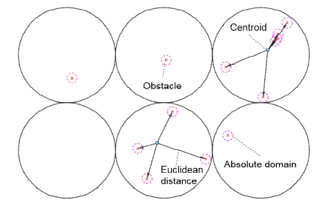
Analysis of obstacles within the assessment area

3.3.3 Coefficient for route risk index

The two coefficients α and β can be calculated by geometrically analyzing the assessment area, and based on the percentage of the non-navigable area within the assessment area. The former is an incremental coefficient derived by the size of the No Go Areas resulting from the shallow water depth, including lands within the circular area. The latter is an incremental coefficient derived by the size of the absolute domain determined by the safe marginal distance within the circular area.

Lastly, coefficient γ is computed by statistically analyzing the influence of weather data on maritime traffic accidents. Korea’s maritime traffic accident data from 2012 to 2016 were collected and analyzed, as listed in Table 2. It was found that among the total of 522 accidents involving grounding, contact, capsizing, and sinking, 112 accidents were influenced by weather factors, including wind, current, and visibility. Therefore, using the concept of the ship’s slip, a new equation to determined the effective influential figure related to γ was introduced. The value of the effective influential figure can be defined as follows:

Table 2

Maritime traffic accident data from 2012 to 2016

(2) EImax=TNAI−NNAENNAE×100

where:

• EI_max = maximum effective influential figure,

• TNAI = Total number of accidents involving weather influence,

• NNAE = Net number of accidents not involving weather influence.

(3) EI=kw⋅w+kc⋅c+kυ⋅υ

where:

• EI = Effective influential figure,

• k_w = weight coefficient of wind factor,

• w = rating of wind factor derived from the matrix,

• k_c = weight coefficient of current factor,

• c = rating of current factor derived from the matrix,

• k_v = weight coefficient of visibility factor,

• υ = rating of visibility factor derived from the matrix.

When Eq. (2) was applied, 27.32% of influential factors were derived by the weather, and this assumes that it is possible to apply EI_max =27.32, and thus, γ_max =1.2732 as the incremental coefficient. Besides, it was analyzed that among the 112 maritime traffic accidents affected by the weather, 78 cases were related to winds, 21 cases were related to currents, and 13 cases involved visibility issues; thus, 0.6964, 0.1875, and 0.1161 portion were applied, respectively for weight coefficient.

Then, the portions were multiplied by 5.464 to obtain the maximum value of EI as 27.32 and weight coefficients based on the assumption that the default value of EI is 0 when there are no weather data. EI can be represented by the Eq. (3). Accordingly, γ value derived by EI would range between 1 and 1.2732 as per the weather factors’ rating found in the matrix and statistical data of the maritime traffic accidents from 2012 to 2016.

4.1 Experimental model

In order to verify the effectiveness of the proposed route risk assessment technique, an experiment was carried out using a model ship carrying HNS. The experiment was conducted in a selected area at the west coastal waters of Korea. A number of ships carrying HNS typically transit in this area to call ports such as Daesan, Pyeongtaek, Dangjin, and Incheon. The developed route risk assessment technique can properly be applied and the reliability of the technique can be verified because there is no traffic lane in this area. Additionally, the selected model ship used in the experiment was a 135K liquefied natural gas (LNG) carrier, as this ship size comprises large portion of the Korean LNG carriers and LNG is one of the major HNS products (Lee, 2004). The following settings were assumed with the model ship steaming speed set at 15 knots, draft at 11 m, block coefficient at 0.68, and 20% margin setting for the No Go Areas were based on the standards considered by most operators (PIANC, 1980). The assessment areas were also drawn in accordance with the position fixing intervals at every 6 minutes according to the definition of the interval.

4.2 Result of the route risk analysis

Prior to plotting a contour map for the experiment area(see Fig. 5), the risk assessment area was designated as per circular areas with a radius of 6-minute-distance, and the No Go Areas in consideration of the maximum draft plus safety margin were identified in gray color and obstacles were marked, as shown in Fig. 6. It was assumed that there was no consideration of time-dependent factors, i.e. tidal height and weather for the purpose of analyzing the result at default. Then, the resulting risk contour showed continuous distribution of the route risk; thus, the officers in charge of route planning or managerial decision makers could easily understand the navigating environment of the corresponding situation.

Fig. 5.

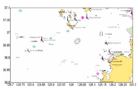
Electronic chart of experimental model area

Fig. 6.

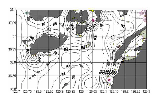
Initial result of the technique application

4.3 Result of the route risk assessment

In the designated area, an experiment was conducted based on two cases. The first was the result of comparison with several routes used by Korean companies operating the model ships under the same condition. Additionally, the same route selected by one company under different conditions was analyzed to verify effectiveness.

4.3.1 Route risk assessment in comparison with several options

After the route risk contour had been plotted, the courses for the model ship to arrive at Pyeongtaek pilot station were drawn. Data regarding the routes leading to this station had been collected from five companies operating LNG ships in Korea (Fig. 7). The routes were divided into two main groups. The result shows that companies A, B, and C followed Group 1 route which is almost a strait line coming from the south-west side of the assessment area. Group 2 route had a relatively larger angle of altering the course and it comes from the middle-bottom side of the assessment area. The graphs represented in Fig. 8(a) and (b) can be visually compared to analyze the routes. Detailed data about each route are also listed in Table 3.

Fig. 7.

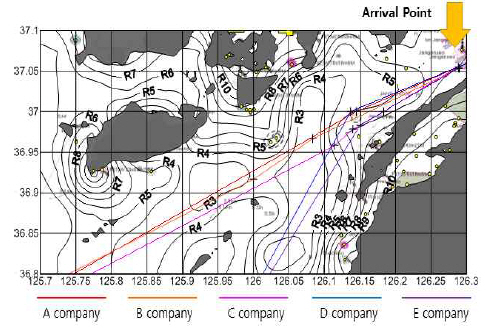
Route risk assessment of diverse route options used by several companies under the same condition

Fig. 8.

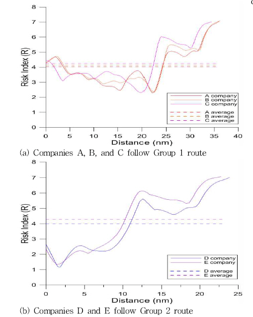
Graphs analyzing the diverse routes based on distance

Table 3

Comparison of the diverse routes

In the designated model area, the routes of companies B and C had relatively more waypoints, while the route of company A had the least number of waypoints. For the distance, the route of company C was the shortest in Group 1, and the route of company E was the shortest in Group 2. Additionally, considering the cumulative risks, which were calculated by the area of the lines from the base, as integration of Fig. 8(a) and (b) illustrated that the route followed by company B had the highest cumulative risks in Group 1, while the company E route had the highest cumulative risks in Group 2. However, to analyze Group 1 and 2 routes based on the same criteria, the cumulative risk value was divided by the distance, to calculate average risk. It was found that the route followed by company D had the lowest average risk, while company C route had the highest average risk. In other words, the route followed by company D is the safest with proceeding distance.

4.3.2 Route risk assessment under different conditions

Finally, the route of company A was compared under different circumstances as shown in Fig. 9(a) and (b). The first one was the default condition, but the second one was the result of reflecting the actual tidal data and weather conditions, which was acquired by a nearby monitoring buoy. At this moment, the tidal height was 5.27 m, and the meteorological condition had 5 ㎧ wind speed, 1 knots current, and 10 nm visibility.

Fig. 9.

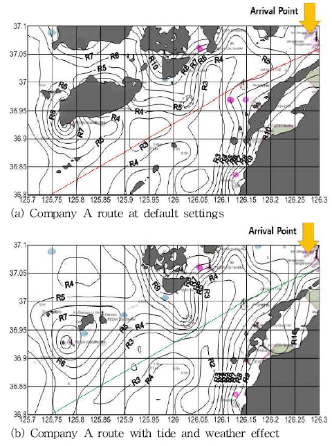
Route risk assessment under different conditions

As a result, not only the whole distribution of the risk contour was observed differently, but also the visualized route risk graph also showed a different trend of values in addition to different No Go Areas, as shown in Fig. 10. It was found that both of cumulative route risk and average risk were significantly reduced to 136.85 and 3.80, respectively, as listed in Table 4. This can be attributed to the tidal height that increased the water depth, and therefore reduced the route risk along the course, although the risk value was relatively higher from 30 nm to the end of the course owing to including the new obstacles, which were previously excluded by the default of No Go Areas. After an observation of the chart, it was also confirmed that the several obstacles such as rocks and buoys were distributed in the area, where those obstacles were not reflected before, because of the No Go Areas.

Fig. 10.

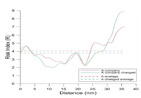
Analysis graph of company A route under different conditions

Table 4

Comparison of company A route under different conditions

4.4 Discussion of the practical applications

The purpose of this study is to quantitatively and visually assess the route risk in the designated area to achieve safe maritime traffic environment at sea. This route risk assessment technique is expected to be applied to the ships carrying HNS to objectively assess the safety of previously planned diverse routes. Furthermore, this technique could be used by officers in charge to determine optimized routes, as company D route had the lowest risks along the course distance, as shown in Table 3. In addition to safety considerations, this approach should consider other relevant factors such as alteration of courses and sailing distance.

Furthermore, this study proposed route assessment based on accident probabilities to prevent maritime traffic accidents beforehand. In fact, the consequential elements can also affect the route risk of maritime traffic accident by ships carrying HNS in consideration of minimizing the impact at preparedness stage once the accident takes place. Furthermore, it was assumed that time-dependent factors such as tides and weather were applied samely in entire the assessment area. Improved result could be obtained if the data for each area is available once the technology allows.

Finally, the application of the developed technique could be expanded to cover wider range of ships, enhance maritime navigation safety, and could further be adapted to autonomous navigation, as it could automatically determine the route by assessing the characteristics of the risk contour map such as gradient and cumulative risks compared to distance in addition to other dynamic factors such as encountered moving ships, which were not considered in this study.