

Introduction
The motion control system of marine vehicles is generally composed of three essential parts which are guidance, navigation, and control systems(Robert et al., 2003). The navigation system is applied to control the marine vehicle by analyzing its dynamic motion states using an optimal route design method(Lee, 2005). The guidance system is employed for the vehicle's motion control, which provides a series of reference inputs continuously to the control system (Bhattacharyya et al, 2014; Gierusz et al., 2007). A trajectory control system(P.H. Nguyen et al., 2006) plays an important role in controlling the motions of the marine vehicle when a series of way points or a path is given. The trajectory control system has an effect on the overall performance and stability of the marine vehicle in practical applications in which various environmental disturbances exist.
This paper mainly deals with a trajectory tracking control method for controlling both speed and heading angle of unmanned ships. There exist various methods for trajectory tracking control especially in shipŌĆÖs autopilot system. In general, the control problem in this case can be handled by separating the surge speed and heading angle (Cimen et al., 2004). In this case, the two different control laws for the surge speed and heading angle are required. This can be regarded as a natural scenario where shipŌĆÖs speed is set to be full speed during voyage on outsea in practical applications. In fact, many researches have been focused on the control algorithm in which surge speed and heading angle are controlled separately (Jun Wu et al., 2012). However, if we concerned with an autopilot system for small-sized ships or unmanned ships, both speed and heading angle should be controlled simultaneously. This is because two control variables are correlated especially in following curved trajectory. In addition, when the ship moves at the narrow water, the surge speed of ship should be controlled (Roberts, 2008).
As a control system for shipŌĆÖs trajectory tracking, sliding mode control theory has been widely studied. Ashrafiuon et al.(2008) proposed a sliding mode control law which was implemented for trajectory tracking of under-actuated autonomous surface ship with camera feedback technology. Cheng et al.(2007) suggested the sliding mode method in which the earth-fix reference coordinates are applied directly to control law. Koshkouei et al.(2007) carried out a comparative study between sliding mode and PID controller in view of the roll stabilization of ships, and concluded that two controllers had their respective advantages. Referring to the aforementioned work, surge speed and rudder angle were assumed to be controlled separately, and the propulsion force and thrust force with respect to a ship were not clearly illustrated. In addition, the relationship between forward speed and thrust was not exposed explicitly.
This paper proposes a SmC(sliding mode control)-based trajectory tracking method for a small-sized unmanned ship to achieve two control objectives(i.e., surge speed and heading angle) in only one control law. To do so, we derive a new control law from a general sliding mode theory, and design a SmC-based controller for shipŌĆÖs trajectory tracking purpose. Furthermore, the propulsion force came from propeller and rudder force caused by rudder are also clarified in this study. The proposed controller is also designed with considering environmental disturbances in order to improve robustness. The performance of our control method is finally evaluated and discussed through a series of simulation results.
This paper is organized as follows. Section 2 describes mathematical models including shipŌĆÖs dynamics/kinematics and environmental disturbance. Section 3 explains the guidance system and the proposed control system. Some simulation results are shown and discussed in section 4, and conclusions are made in section 5.
mathematical models
2.1 Ship model
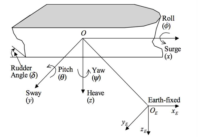
Even though a marine vehicle has 6-DOFs(degrees of freedom) motions, only the ship motions on the horizontal-plane are generally considered for coursekeeping or track-keeping problem in practical applications. Due to that, 6-DOFs model is simplified to 3-DOFs model in this paper.
Ship dynamics is obtained by applying NewtonŌĆÖs laws. In this paper, it is assumed that i)the coordinate of body-fixed frame origin is placed in the center line of the ship (yG = 0), ii)the mass distribution is homogeneous, and iii)the xzŌĆöplane is symmetrical, and iv)the influence of motion in zŌĆödirection (heave) and rotational motions by x ŌĆöaxis(roll) and yŌĆöaxis(pitch) are neglected. Then, the nonlinear dynamic ship model can be linearized by the additional assumption that higher order perturbation can be neglected. The external force X , Y , N are considered as the forces along x-axis, y-axis and moment along with z-axis respectively (Lee, 2005 and Chae, 2016). The disturbance force caused by environment is described in section 3.2. Let X u ╦Ö , X u , T
where t and Tloss stand for thrust deduction number and loss term (or added resistance), respectively. We put these two factors into nonlinear part of state space equation.
The linear steering dynamics is written as;
where the symbols Y Žģ ╦Ö , Y r ╦Ö , N Žģ ╦Ö , N r ╦Ö
For a ship moving at constant path, the variation of rudder angle is small, which results in the following approximations:
Therefore, the rudder force and moment are expressed as
The the parameters Y╬┤ and N╬┤ are defined by
where ╬┤ is angle of rudder, A╬▒ is area of shipŌĆÖs stern, and UR is flow speed of sea water passing through the rudder. In practice, UR has a little bit difference with total speed of ship, thus we consider it as the total speed. The symbol xR is distance from the gravity center to the stern, Žü is density of seawater, and ╬ö is the ratio between the height of ship and beam of ship. Hence, the equations of shipŌĆÖs steering motion can be written as (13)-(15).
Here, ╬ø= [v, r]T and b= [Y╬┤ , N╬┤]T . The symbol n stands for the revolution of the propeller, ╬┤ is angle input for steering engine, and u0 and v0 are the nominal surge and sway speed of ship, respectively. Also, M and N are denoted by inertia matrix and hydrodynamic damping matrix.
Combining the speed equation and steering equations into one equation, the ship's dynamic equation can be described in state space form of
In (16), the function f(x) is related to the nonlinear part that involves the thrust deduction number, loss term, and external disturbances.
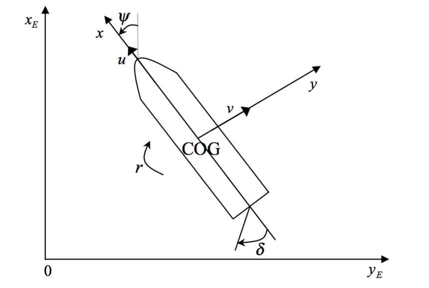
The above dynamic equations are based on the body-fixed frame. In consideration of kinematics equations, the earth-fixed frame as shown in Fig. 2 should be considered. In order to transform the state variables from the body-fixed frame to the earth-fixed frame, a 3-DOFs transformation matrix is employed as expressed in (28).
2.2 Environment Disturbance model
The types of environmental disturbances can be divided into wave, wind, and ocean current. Among many possible external disturbances acting on a ship, only a disturbance is considered in this paper. Since the wave caused by wind influences the performance of the autopilot system dominantly, the other environmental disturbances are neglected in this paper. The wave model can be described by (Fossen, 1994)
where w (s) is a zero-mean Brownian process noise. The function h(s) is second order wave transfer function which is expressed as
where w0 , ╬Č, and Kw are a wave frequency, a damping coefficient, and a gain constant. Here, the gain constant is defined by Kw = 2╬Čw0Žām where Žām is the wave intensity. The wave frequency generated by wind for Pierson-moscowitz sepectrum is defined by
where V is a wind speed and g is acceleration of gravity. For a ship moving with forward speed U , the wave frequency w0 is modified to encounter frequence we as (32).
Here, g is the acceleration of gravity, U is the total speed of ship, and ╬▓ is the angle between the heading and the direction of the wave. Considering the encountered frequency, wave model can be derived as (33).
Here, wh is white Gaussian noise. In this model, the frequency of motion caused by the wave is much higher than the bandwidth of the controller. By appling the wave model, the shipŌĆÖs final heading angle, which is influenced by wave, is determined from (35).
SmC-based tracking controller
In this paper, a waypoints-based method is employed as a guidance system to lead the ship to the path by computing the desired heading angle. Since such a guidance system can be simply implemented, this paper concentrates more on the trajectory control system.
A sliding mode control is known well as a robust control methodology which can be applied to nonlinear control systems in practical applications. In the shipŌĆÖs trajectory control field, the sliding mode control also can be applied. However, trajectory tracking involves forward thrust part used to control surge speed and the rudder control part applied to minimize tracking error. This requires to control the propulsion force and rudder angle at same time. Other researchers generally utilized the separated control laws to remedy such an issue. This paper proposes an alternative to control both speed and angle by only a control law. In order to realize it, regarding HealeyŌĆÖs sliding method as an original method and referring to the sliding mode control of invertible systems, we modify the original one by using vector method to extend the control input dimensions. To illustrate, the Healey's SmC is also called SmC using eigenvalue decomposition, as the name implied, in this method, pole placement method is applied to obtaining the desired eigenvalue in order to simplify the control algorithm. In addition, using pole placement method to choose the proper pole can make the state variable stable at the steady-state response. The sliding mode control of invertible systems was investigated by Tustomu mita (Bartolini et a.l, 2009).
3.1 modified SmC algorithm
The modified sliding mode control is described as follows. Let x ╦£ x ╦£ = x ŌłÆ x d
where h is multiple dimensions matrix. In fact, it is h(ŌłłŌäØn ├Śp) matrix where p indicates the number of the control input (for example if we want to define the number of control input as 3, then we can set p=3). In this way, Žā would become a Žā(ŌłłŌäØp├Ś1)matrix. Using the SmC, we want the sliding surface to approach to zero, which indicates the error(x ╦£
We assume that the dynamic and kinematic model are described as
where x(ŌłłŌäØn)ŃĆĆandŃĆĆq(ŌłłŌäØ) .The function f(x) should be interpreted as a nonlinear function that describes the deviation from linearity in terms of disturbances and unmodeled dynamics. In this paper, these disturbances are the deviation of parameters in the state equation caused by surge speed variation. In addition, the experiments of Healey and co-authors showed that this model could be used to describe a large number of vessel conditions. The feedback control law is composed of two parts
Compared with the original one, the feedback control law becomes a vector. This can be written in the matrix form of q(ŌłłŌäØp├Ś1) , and the nominal part is chosen as
where k is the feedback gain vector. Substituting (39) into state equations, we yield the closed-loop dynamics:
In this way, we can obtain the desired eigenvalue of Ac by adjusting gain value of k using pole placement method.
To prove convergence of Žā, the Lyapunov candidates function is applied in form of
Differentiation of V(Žā) with respect to time must meet
Because only if differentiation of V(Žā) is negative, the sliding surface can approach to zero which means lim Žā t ŌåÆ Ōł× = 0
To make (44) simplified, we choose q (assuming that hŌŖżB ŌēĀ 0) as
where f ^ ( x ) Žā ╦Ö
where ╬ö f ( x ) = f ( x ) ŌłÆ f ^ ( x ) A c T h
where ╬╗(Ōłł╬╗(A)) is an eigenvalue of Ac and m is called to be a right eigenvector of Ac for ╬╗. This trick indicates that if the eigenvalue is equal to zero, the A c T h
where ╬╗i (ŌłĆi = 1,...,p) = 0 while hj (ŌłĆj = 1,...,p) consists of specific values. We can compute h by
where h = { h j | j = 1 , ... , p } A c T A c T h
Because the sliding surface is multi-dimension vector, sgn(Žā) should replace by Žā ŌĆ¢ Žā ŌĆ¢
Due to globally- and asymptotically-stable conditions, ŌŖż must be selected to meet
Hence, in order to make sliding space asymptotic, we must ensure ŌŖż to meet the following requirement as (53).
This method is similar to HealeyŌĆÖs SmC theory in which the control input is dealt with only for one dimension. However, our method can be extended to multiple dimensions so that we can design a general controller regardless the number of control inputs.
3.2 Design of trajectory tracking controller based SmC
When the proposed control algorithm is employed to handle with the problem stated in this paper, according to practical conditions, the control inputs are selected by rudder angle and revolution of engine. We choose the state variable as
The nonlinear part is shown as following, and wn is environment noise following gaussian distribution.
Therefore the control law is derived from (58).
Here, x is state vector of ship model, k is constant matrix obtained by pole-placement algorithm, and h is constant matrix obtained by (34). Also, q1 is revolution of engine (unit: rps) and q2 is the rudder angle (unit: radian).
In this paper, we assume
where T ^ l o s s Žł ^ w a Žģ e
Simulation results
4.1 Simulation setup
Our target ship is a small-sized ship whose length and beam are 10m and 5m, respectively. For simulations, we utilized the model parameters by referring to the Prime System as follows: Table 1
Table┬Ā1
Parameters of ship
With those ship model parameters, the control law could be calculated by using (59). The desired route was divided into a set of points so that it was convenient to apply way-points method for obtaining the designed angle. In fact, this angle is regard as the control input for the sliding mode controller. In this simulation, the wave disturbance induced by wind was considered. We also used the wave state space model to put influence on heading angle. The wave model parameters used in the simulation were set to be ╬Č = 0.1, we> = 1.1, Kw = 10, and wh Ōł╝N (0 ,0.03) , respectively.
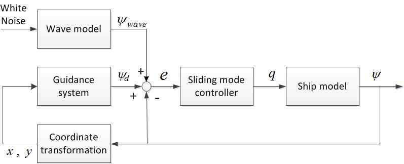
Fig. 3 depicts the procedure of trajectory tracking control for the target ship. In this figure, ╬”d = [vd,Žłd] represents a reference vector consisting of desired speed(vd) and heading angle(Žłd), which can be determined by the guidance system. The SmC-based control system outputs revolution(n) and rudder angle(╬┤) acted on the ship model, from the error vector(e) input. Heading angle of ship is affected by the wave, which is considered as the feedback. The output vector is modified by the transformation matrix, and earth coordinates are generated.
4.2 Heading angle and speed control simulation
We verified the steering control and surge speed control firstly. The initial condition of shipŌĆÖs speed and heading angle were zeros. We set two constant desired values as speed command and heading angle command to validate the performance of SmC controller under the disturbance caused by environment noise.
Fig. 4 shows the simulation results of steering control. In this simulation, the desired heading angle of ship was 1.55 radians that means 100 degrees. After 60 seconds, the heading angle reached at the desired angle. The heading angle shows stable since the disturbance including wave force rejected by control inputs. The rudder angle regarded as the control input of steering control is shown in Fig. 5. The variation of rudder angle is not smooth from 75 seconds. At this point the heading angle and surge speed are converged to desired value.
Fig.┬Ā4.
Simulation result of heading angle control: the top is the variation of heading angle and the bottom is variation of rudder angle considered as control input
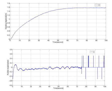
Fig.┬Ā5.
Simulation result of speed control: the top is surge speed of ship and bottom is engine rpm
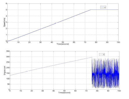
Fig. 5 displays the situation of speed control. In this simulation, the desired speed was 5m/s, and surge speed of ship approached to the desired value within 75 seconds, after that the surge speed was stable. For the real ship using the diesel engine, we controlled the surge speed by adjusting the revolution of shaft in practice. The revolution unit is rpm(revolution per minute). As shown in Fig. 5, the revolution increased when the ship is just started. After the ship moved at constant speed, the control input was changed to bang-bang control for rejecting disturbances. Due to the good robustness of proposed SmC, surge speed deviation was near zero. This results present that the speed can be controlled well with steering control together.
4.3 Ship's trajectory control simulation
The next simulation is related to shipŌĆÖs trajectory tracking control. A way-point method was applied to the simulation. In this simulation, the influence of noise was eliminated by controller instead of low pass filter. Also, six points of path were used as a series of way points that are (250,0), (250,700), (700,700), (700, 500), (500, 250) and (625, 125), respectively. ShipŌĆÖs initial position was set to be (0, 0). In addition, the environment noise was imposed during the process of simulation. In order to validate the speed control performance, the ship moved at slowly speeds on every turning. The results are described at from Fig. 6 to Fig. 8.
Fig.┬Ā6.
Simulation result of ship's trajectory control: the dotted line is reference trajectory and full line is ship's path
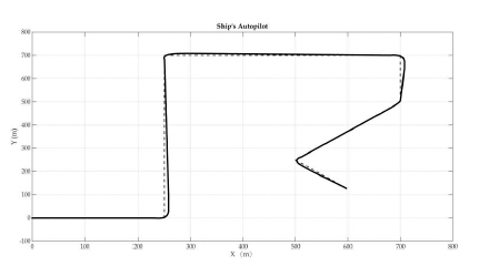
Fig. 6 depicts the shipŌĆÖs path on 2-dimensional space. Based on our way-point strategy, after the shipŌĆÖs position approached to the designed point, the next point was selected through the guidance system. In this manner, the target ship could move along the given path with slight cross-tracking error as shown in Fig. 6. In addition, SmC-based controller suppressed the affect caused by environment noise effectively.
Fig. 7 shows the variation of heading angle. The heading angle is changed efficiently during turning, which implies that the SmC-based controller works well. In this simulation, the behaviour of the target ship was designed to move at slow speed on the turning. Initial speed and general speed were set to be 0m/s and 5m/s, respectively. We also confirm that the ship could move at the desired speed as we expected. Consequently, it is confirmed that the proposed SmC controller and guidance system can be applied to carry out shipŌĆÖs trajectory control task precisely and efficiently.

Conclusions
This paper has dealt with ship's speed and heading angle control that could cope with the ship's trajectory control problem. In our ship model, the prolusion force came from propeller and rudder force caused by rudder were clarified. The environment disturbance especially for wave caused by wind was also involved in the ship model. In order to control surge speed and heading angle simultaneously, a modified sliding mode control law was proposed. The proposed method was tested through a series of simulations based on the linear ship model and a way-point guidance framework. As the simulation results showed, for the speed and heading angle control, the error deviation was close to zero. For ship's trajectory control, we confirmed that the target ship could pass through the way-points accurately and shipŌĆÖs speed could be controlled as we expected.
Although the effectiveness of the proposed method was verified through realistic simulations, it would be required to test through real situations. Further work includes such experiments together with enhancing our method.
 PDF Links
 PubReader
 Full text via DOI
 Download Citation
 Print
Print